SAS to R Migration: How to Import, Process, and Export SAS Files in R

UPDATED: June, 2026 by Vedha Viyash.

When it comes to data analytics, it's no secret that R gives you way more bang for your buck than when compared to SAS.

R won't cost you a penny, but the same can't be said for SAS licenses. In addition, R gives you access to thousands of packages created by other data scientists who've probably already solved the exact problem you're dealing with. Plus, when you need help, there's a huge community ready to jump in with answers on places like Stack Overflow or GitHub.

The case for R now reaches well beyond cost and convenience. Regulators have come around too. The R Consortium's R Submissions Working Group has now completed a series of pilot submissions to the US FDA built entirely in R, covering tables and figures, a Shiny app, ADaM datasets, and containerized/WebAssembly delivery. In 2025 the FDA also expanded the file types its electronic gateway accepts to include R-specific formats, making R a fully viable language for regulatory work, not just internal analysis.

Why does this matter to you? If you're working at a company that's been using SAS forever but wants to modernize, you can't just flip a switch overnight. You need both systems to play nice during the transition, letting you leverage your existing SAS files while building new workflows in R.

SAS vs R Programming: Which to Choose and How to Switch

In this article, we'll show you exactly how to read, manipulate, and write SAS files in R, plus how to go a step further and produce regulatory-grade outputs, so you can seamlessly bridge these two worlds.

Table of contents

• Introduction to SAS
• How to Read SAS Files in R
• How to Save R DataFrames to SAS Files
• Beyond .xpt: CDISC Dataset-JSON, the Modern Transport Format
• Example: Aggregate SAS File in R
• R and SAS Best Practices
• Summing up R and SAS

Introduction to SAS

SAS (Statistical Analysis System) has been the go-to analytics software for many large enterprises and government agencies since the 1970s. It's especially common in regulated industries like healthcare, finance, and pharmaceuticals where reputation for stability and validation matters the most.

This doesn't mean large companies aren't transitioning to open-source. Read this recent exampl

• GSK's Open-Source Shift: Training 1,000 Biostatisticians in R

But what exactly makes SAS different from R? The biggest distinction is that SAS is a commercial, proprietary software with a focus on enterprise-level data processing. You'll find it's great at handling massive datasets and comes with excellent technical support — if you can afford the hefty price tag.

Many organizations have built their entire data infrastructure around SAS. This means there's tons of legacy data stored in SAS formats that you'll need to access even as you transition to R. That's why knowing how to work with SAS files is an essential skill in your data science toolkit.

Beyond SAS: How R is Revolutionizing Pharma and Life Sciences

Different SAS file types

Before we dive into the code, let's understand what we're working with. SAS uses a couple of different file formats, but these are the two you'll encounter most often:

• SAS Data Files (.sas7bdat) - These are the bread and butter of SAS, similar to data frames in R. They store tabular data with rows and columns, including numeric, character, and date variables. Think of them as Excel.
 
• SAS Transport Files (.xpt) - These are platform-independent files designed for sharing SAS datasets between different systems. They're handy when you need to transfer data between SAS and other software like R.

There are other SAS file types too, like catalog files (.sas7bcat) that store metadata, but you'll be dealing with .sas7bdat and .xpt files most of the time when working between SAS and R.

Now that you understand what you're working with, let's look at how to actually read these files in R.

Open-Source Adoption in Pharma: Opportunities and Challenges

How to Read SAS Files in R

Reading SAS files in R is easy thanks to the {haven} package, part of the tidyverse ecosystem. First, you'll need to install it if you haven't already:

install.packages("haven")

Once installed, load the package and use the read_sas() function to import your SAS data file:

library(haven)

# Dataset: https://github.com/RhoInc/sas-codebook/blob/master/ExampleFiles/cars.sas7bdatsas_data <- read_sas("data/cars.sas7bdat")

head(sas_data)

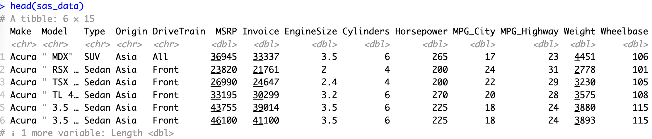
That's it! Your SAS dataset is now available as an R data frame (technically, a tibble). The head() function gives you a quick peek at the first few rows of your imported data.

For this example, we've used a cars dataset that's freely available on GitHub. Feel free to download it if you want to follow along with the code.

Encoding issues

Sometimes you'll run into encoding problems when importing SAS files, especially if they contain special characters or were created in a different locale. If you see weird symbols where characters should be, try specifying the encoding:

read_sas("data/cars.sas7bdat", encoding = "UTF-8")

Common encodings include "UTF-8" (the most universal), "latin1" (common in Western Europe), and "windows-1252" (common on Windows systems). You might need to try a few different options depending on how your SAS file was created.

Dealing with SAS labels

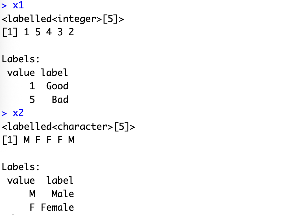
One of SAS's distinctive features is its labeling system. SAS uses labels to attach metadata to values, which is different from how R handles factors. The haven package provides a special function called "labelled" to help bridge this gap.

Here's a simple example of how labelled vectors work in R:

x1 <- labelled(
    sample(1:5), 
    c(Good = 1, Bad = 5)
)
x2 <- labelled(
    c("M", "F", "F", "F", "M"), 
    c(Male = "M", Female = "F")
)

You can then include these labelled vectors in a data frame (or tibble):

library(tibble)

tibble(x1, x2, z = 1:5)

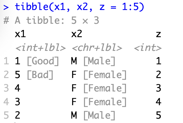
When haven imports a SAS dataset with labels, it automatically converts them to this labelled class. This preserves the original information while making it accessible in R.

How to Save R DataFrames to SAS Files

Once you've done your data manipulation in R, you'll often need to send the results back to colleagues who are still using SAS. The haven package makes this possible, but there's a crucial distinction you need to understand first.

Here's a critical warning about exporting to SAS: Even though haven offers two export functions, only one of them actually works reliably. The write_sas() function attempts to create native .sas7bdat files, but since the SAS format is proprietary and poorly documented, these files often can't be opened by SAS itself. Always use write_xpt() instead, which creates SAS transport files (.xpt) that SAS can consistently read without issues.

In other words, if you want your SAS colleagues to actually be able to open your files, use write_xpt() instead of write_sas(). Here's how to do it:

my_data <- data.frame(
    ID = 1:5,
    Name = c("Bob", "Ed", "Rod", "Dav", "Eva"),
    Value = c(90, 85, 78, 92, 88)
)

write_xpt(
    my_data,
    path = "data/output_file.xpt"
)

# Confirm
read_xpt("data/output_file.xpt")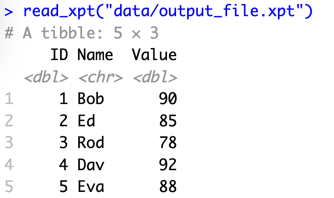

The code above creates a simple data frame with three columns and then exports it as a SAS transport file. The last line reads the file back in to confirm that the export worked correctly.

Writing submission-grade .xpt files with xportr 

There's an important caveat to the workflow above. write_xpt() is perfect for casually handing data to a SAS colleague, but it is not enough to produce a transport file that meets CDISC submission requirements. R data frames don't carry the variable labels, per-variable lengths, types, formats, and column ordering that regulators expect, and write_xpt() won't add or check them for you.

That's where xportr comes in. It's an open-source package (part of the pharmaverse, co-developed by GSK, Atorus Research, and Appsilon) that sits on top of haven and applies CDISC metadata and compliance checks before writing the file. Where haven is the general-purpose reader and writer, xportr is the submission-grade finishing layer.

You drive it with a metadata specification and a short pipeline of functions, each applying one piece of the required metadata:

# install.packages(c("xportr", "pharmaverseadam", "metacore"))

library(dplyr)
library(xportr)
library(pharmaverseadam)
library(metacore)


load(metacore_example("pilot_ADaM.rda"))        # loads an object called `metacore`
adsl_spec <- metacore |> select_dataset("ADSL")


pharmaverseadam::adsl |>
  xportr_metadata(adsl_spec, "ADSL") |>
  xportr_type() |>
  xportr_length() |>
  xportr_label() |>
  xportr_order() |>
  xportr_format() |>
  xportr_df_label() |>
  xportr_write("adsl.xpt")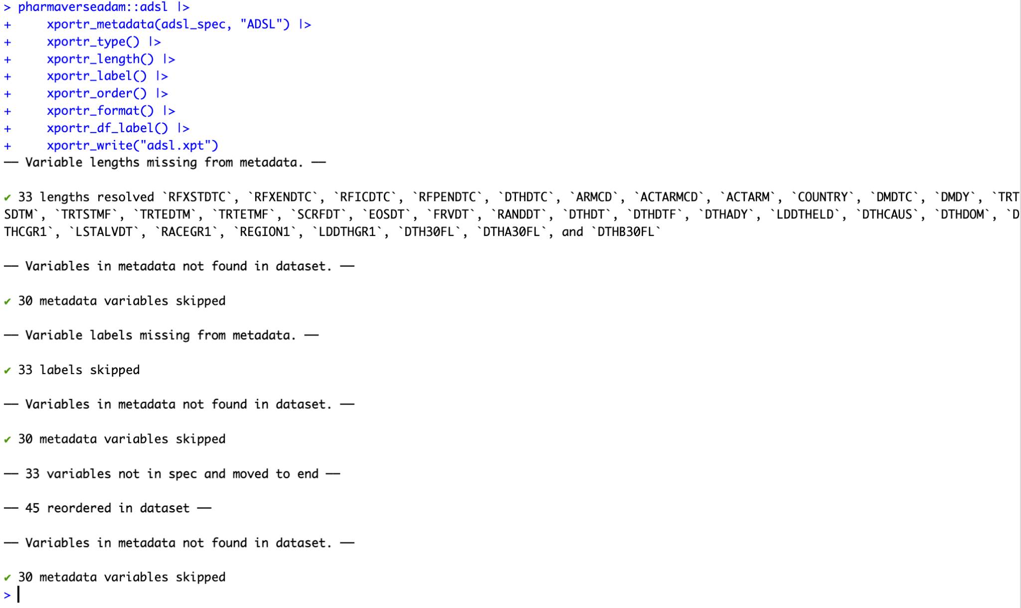

Along the way, xportr warns you about common compliance problems (variable names that are too long or don't start with a letter, character columns wider than 200 bytes, missing labels) so you catch them before the file ever reaches a validator like Pinnacle 21 or a regulatory reviewer. If you're producing SDTM or ADaM datasets for an actual submission, this is the function set you want, not bare write_xpt().

Handle missing values

R and SAS handle missing values differently. In R, we use NA, while SAS has multiple types of missing values. The haven package lets you work with these differences through the tagged_na() function:

my_data <- data.frame(
    ID = 1:5,
    Name = c("Bob", "Ed", "Rod", "Dav", "Eva"),
    Value = c(90, 85, 78, 92, 88),
    na_values = tagged_na("Not applicable")
)

write_xpt(
    my_data,
    path = "data/output_file_with_na.xpt"
)

# Confirm
read_xpt("data/output_file_with_na.xpt")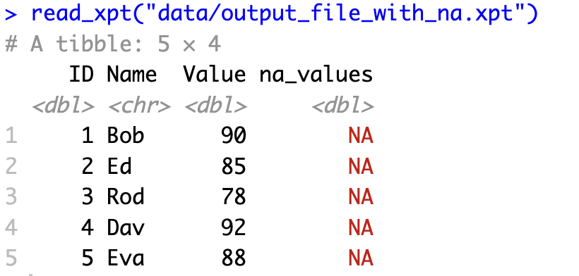

This approach lets you preserve the meaning behind different types of missing values when moving between R and SAS. For example, you might want to distinguish between "Not applicable," "Refused to answer," and "Don't know" in survey data.

When you read this file back into R, you'll see the tagged NA values preserving the original information. Similarly, when your SAS colleagues open the file, they'll see the appropriate missing value codes.

Now that you know how to both read and write SAS files in R, let's put these skills together in a practical example.

Beyond .xpt: CDISC Dataset-JSON, the Modern Transport Format

Everything above relies on the SAS V5 transport (.xpt) format. It's worth understanding why that format exists, and why the industry is moving past it.

The V5 transport format dates back to SAS version 5 in the 1980s, and it shows its age. It imposes some hard limits that are painful in modern clinical data: variable names capped at 8 characters, labels capped at 40 characters, character fields capped at 200 bytes, and US-ASCII only, which means no native support for Unicode or multibyte text such as Japanese or Chinese. It's also storage-inefficient, often wasting a large fraction of file size on padding.

Enter Dataset-JSON, a CDISC standard built specifically to replace the V5 transport format. As the name suggests, it stores tabular clinical data as JSON, which makes it tool-agnostic (no SAS required to read or write it), Unicode-friendly by default, far more compact, and able to link out to a Define-XML document for richer metadata. CDISC published Dataset-JSON v1.0 in 2023 and the more complete v1.1 in December 2024.

Why this matters now: the regulatory picture

This isn't just a technical curiosity. On April 9, 2025, the FDA published a Federal Register notice stating that it is exploring CDISC Dataset-JSON v1.1 as a new exchange standard, with the long-term potential to replace SAS V5 XPT for submissions to CDER and CBER. That followed a 2022 FDA assessment that identified JSON as the optimal modern format, and a 2023–2024 FDA/CDISC/PHUSE pilot that concluded Dataset-JSON could serve as a transport format for study data.

One caveat worth stating plainly: as of mid-2026, Dataset-JSON is still under evaluation. It is not yet in the FDA Data Standards Catalog, and XPT v5 remains the required transport format for submissions today. The trend is clear, but for now the sensible approach is to keep producing compliant XPT for your submissions (with xportr) while piloting Dataset-JSON in parallel, so you're ready when the catalog changes.

Reading and writing Dataset-JSON in R

R already has tooling for this, via the datasetjson package (from Atorus Research, available on CRAN). Current releases target the v1.1 version of the standard. The package lets you construct a Dataset-JSON object from a data frame, attach the required study and dataset metadata, and read or write the file:

# install.packages("datasetjson")
 
library(datasetjson)
 
# 'iris_items' is example variable metadata bundled with the package,
# so no column spec needs to be built by hand.
ds <- dataset_json(
    iris,
    item_oid  	= "IG.IRIS",
    name      	= "IRIS",
    dataset_label = "Iris",
    columns   	= iris_items
)
 
# Write to disk, then read it back
write_dataset_json(ds, file = "iris.json")
df <- read_dataset_json("iris.json")

The columns metadata (variable names, labels, data types, lengths) is required by the standard. The package vignette walks through building it, and it maps neatly onto the same specification you'd use to drive xportr. In other words, once you maintain dataset metadata properly, you can emit either an XPT file for today's submissions or a Dataset-JSON file for the format that's coming next.

Exploring the Top 5 pharmaverse Packages

Example: Aggregate SAS File in R

Let's put everything together with a practical example. One common task when transitioning from SAS to R is recreating your SAS summary reports in R and then sharing the results back with your SAS-using colleagues.

We'll use the cars dataset again, group it by vehicle type, and calculate summary statistics - similar to what you might do with PROC MEANS in SAS.

First, let's import the data and create a summary report with the summarytools package:

library(dplyr)
library(summarytools)
    
data <- read_sas("data/cars.sas7bdat")
grouped_data <- data %>%
  group_by(Type)
    
view(dfSummary(grouped_data))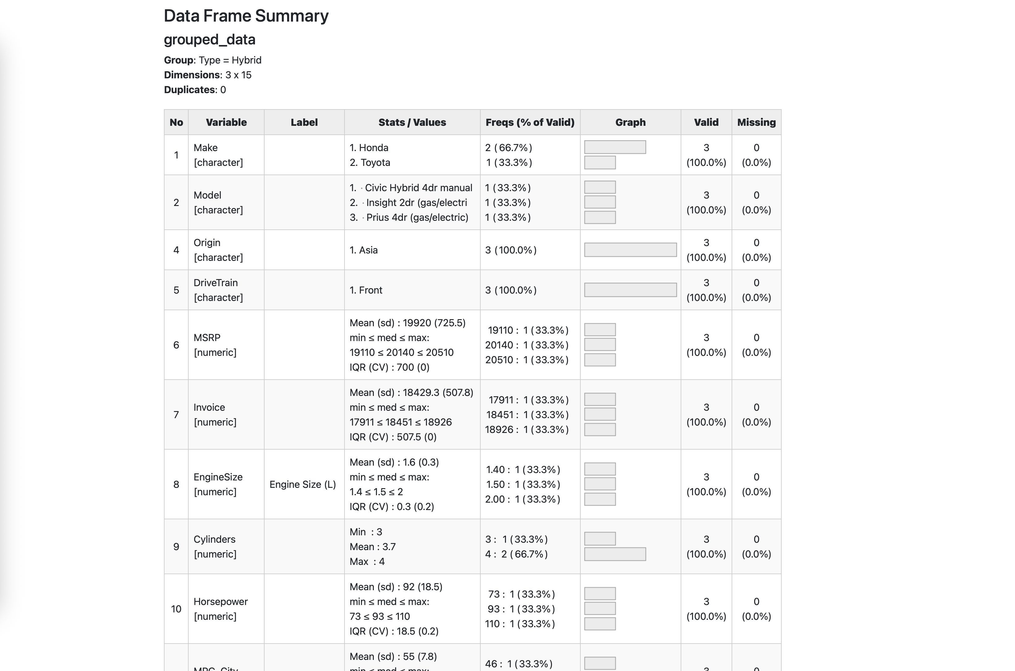

The code above will open an HTML report in your viewer pane and show detailed statistics for each variable in the dataset, grouped by the vehicle type. In other words, ut's a quick way to get a comprehensive overview of your data.

But what if you want more control over exactly which statistics to calculate? Let's create a custom summary and export it back to SAS format:

summarised_data <- data %>% 
  group_by(Type) %>% 
  summarise(
    across(
      where(is.numeric),
      list(
        mean = mean,
        stdev = sd,
        median = median,
        min = min,
        max = max,
        iqr = ~IQR(..1, na.rm = TRUE)
      )
    )
  )
  
summarised_data
  
write_xpt(
  summarised_data,
  path = "data/cars_summarised.xpt"
)

This more advanced example uses dplyr's powerful across() function to apply multiple summary statistics to every numeric column in our dataset. Here's what's happening:

• We group the data by vehicle type.
• We use summarise() with across() to apply functions to multiple columns at once.
• where(is.numeric) selects only the numeric columns.
• We apply six different statistics to each numeric column.
• Finally, we export the result as a SAS transport file.

The result is a  summary table with columns named like "MPG_City_mean", "MPG_City_median", etc. This gives you a similar output to what you'd get from PROC MEANS in SAS, but with the flexibility and power of R's data manipulation tools.

If your SAS colleagues need this summary data for further analysis or reporting, they can import the .xpt file using standard SAS code like:

libname mylib xport "path/to/cars_summarised.xpt";
data work.cars_summary;
  set mylib.summarised_data;
run;

And that's all there is to it!

R and SAS Best Practices

Transitioning from SAS to R won't always be smooth sailing. Hopefully, you can minimize risks by following these best practices:

   
• Document everything: Use R Markdown or Quarto to create reproducible reports that track how you processed the data. This is crucial when transitioning between systems and helps both you and your colleagues understand each transformation step.
   
• Handle missing values properly: R and SAS treat missing values differently. Be explicit about how you want to handle NAs when moving between systems, especially if certain missing values have specific meanings in your data.
   
• Test your workflow: Always verify that your exported SAS files can be read correctly by having a SAS user try to open and use them. This simple step can save hours of troubleshooting later.
   
• Seek help: If you require further guidance, don't hesitate to seek help from the Posit community or SAS communities. Collaboration can often lead to quicker solutions.

Summing up R and SAS

We've covered a lot of ground in this guide to working with SAS files in R. You now know how to import SAS datasets into R, process them, and export the results back to SAS format for your colleagues.

The haven package makes this cross-platform workflow possible, and it gives you the freedom to use R's flexibility while still collaborating with teams that rely on SAS. Remember to use read_sas() for importing and write_xpt() (not write_sas()) for exporting to ensure maximum compatibility.

If you're in the middle of a SAS to R migration at your organization, this hybrid approach lets you gradually transition workflows without disrupting existing processes. You can start building new analysis in R while maintaining compatibility with legacy SAS systems.

Want to get more out of your data with custom analytics solutions? We're here to help you modernize your data workflow. Whether you're just starting your SAS to R migration or looking to enhance your existing R capabilities, our team of experts can guide you through the process.

Reach out to Appsilon to transition from SAS to R